
Optional Lab: Model Representation
Based on Optional Lab 02 (Week 1, Course 1) of the Machine Learning Specialization, by Andrew Ng (DeepLearning.AI / Stanford). But forget the notebook for a second, let's actually understand what's going on.
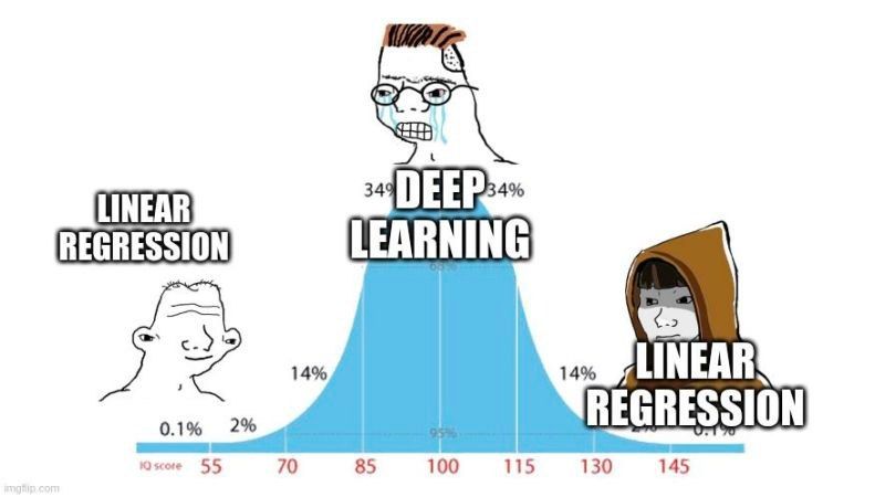
Here's the thing: everyone getting into ML hears about neural nets, transformers, LLMs, all the hyped-up stuff. Then you open the first lab of the most recommended course in the field and find... a line. y = ax + b from middle school, just with the variable names swapped around.
That's not the course stalling before the "real" material. This is the real material. Linear regression is the base Lego brick: every fancier model you'll study later (neural nets, logistic regression, whatever comes next) is, underneath, a pile of these bricks stacked up. Understanding this one down to the bone taught me way more than memorizing a neural net formula without knowing where it came from.
What you'll walk away knowing
- Why we represent training data as a NumPy array instead of a plain Python list.
- How to count how many training examples you have () and grab a specific one.
- Why looking at your data before modeling isn't a "nice to have", it's a survival rule.
- How to build the model in code.
- How to play with the parameters until you nail the perfect fit, by hand, no magic formula, and feel firsthand why that doesn't scale.
Every supervised model has three pieces: the data, the model function, and the parameters. This post puts all three together in the simplest version that exists. Hold on to that structure: it comes back, just bigger, in pretty much everything else this course covers.
The field's dictionary
ML has an annoying habit of inventing symbols for simple things. Here's the "dictionary" the course uses, since it carries through everything that follows:
| Notation | What it is | In Python |
|---|---|---|
| a plain number (scalar) | - | |
| a list of numbers (vector, bold letter) | - | |
| the input values of every training example | x_train | |
| the values we're trying to predict, for every example | y_train | |
| , | the pair of values for example number | x_i, y_i |
| how many training examples you have | m | |
| weight (the line's slope) | w | |
| bias (where the line starts) | b | |
| what the model predicts for example | f_wb |
Two mix-ups that trip up every beginner:
- is not a power. That
(i)in parentheses just means "which row in the table", an index. is the third example (remember, we count from zero), while would mean "x squared", a completely different thing. - is the number of rows (examples). Later on shows up, the number of columns (features). Think of a spreadsheet: is how many houses you've logged, is how many columns of information you tracked about each one (size, bedroom count, neighborhood...). Here we've only got one column, so .
The problem: what's this house worth?
Scenario: you're a real estate agent with exactly two closed sales so far. One house at 1000 sqft sold for 500k. A client shows up with a 1200 sqft house asking what it's worth. You don't have a crystal ball, but you have two data points, and it was surprising how much I managed to pull out of that.
To avoid writing a pile of zeros, size becomes "thousands of sqft" and price becomes "thousands of dollars":
| Size (1000 sqft) → | Price (1000 dollars) → | |
|---|---|---|
| 0 | 1.0 | 300 |
| 1 | 2.0 | 500 |
So: examples, and .
My plan was to fit a line through (or close to) those points. Once we find that line (i.e. once we find and ) we can estimate the price of any new house, including one we've never seen, like that 1200 sqft one.
Smaller scales are a habit, not just tidiness: later in the course, once the numbers get genuinely large, normalizing scales (feature scaling) becomes essential for training to not stall or blow up. Start getting your eye used to it now.
Put it in an array
# =====================================================================
# TRAINING DATA
# =====================================================================
# x_train -> INPUT variable (feature): house size, in thousands of sqft
# y_train -> TARGET variable:          house price, in thousands of dollars
# Order matters: x_train[0] and y_train[0] describe the SAME house.

x_train = np.array([1.0, 2.0])       # Creates a 1-D NumPy array with the two sizes.
y_train = np.array([300.0, 500.0])   # Creates a 1-D NumPy array with the matching prices.

print(f"x_train = {x_train}")
print(f"y_train = {y_train}")
Output:
x_train = [1. 2.]
y_train = [300. 500.]
Notice I used np.array, not a plain Python list ([1.0, 2.0] on its own). That's not fancy-library snobbery: a NumPy array keeps the numbers packed tightly in memory and runs math on all of them at once (this is called vectorization), instead of looping item by item the way a list would. With 2 numbers it makes zero difference, but with 2 million it's the difference between running in seconds or freezing your machine. The entire course, and honestly most serious ML code, starts from NumPy because of exactly this.
On f-strings: the
fbefore the quotes means Python evaluates whatever's inside{ }and drops it into the text.{value:.2f}formats with 2 decimal places. You'll see this everywhere from here on out.
How many examples do I have? ()
# Via .shape -- returns a TUPLE with the size of each dimension.
print(f"x_train.shape: {x_train.shape}")   # (2,) for a 1-D vector with 2 elements.
m = x_train.shape[0]
print(f"Number of training examples is: {m}")

# Via len() -- works on NumPy arrays just like it does on lists.
m = len(x_train)
print(f"Number of training examples is: {m}")
Both give the same result here, but I picked up the .shape habit early, and it's worth picking up too: once your data has multiple columns (that shape mentioned above), .shape tells you rows and columns up front, while len() only gives you the row count and leaves you guessing about the rest.
Grabbing a specific example
Python counts from zero, always:
| Index | In Python | |
|---|---|---|
| 0 | x_train[0], y_train[0] | |
| 1 | x_train[1], y_train[1] |
i = 0                    # Index of the example we want to inspect.
x_i = x_train[i]
y_i = y_train[i]

print(f"(x^({i}), y^({i})) = ({x_i}, {y_i})")
Output:
(x^(0), y^(0)) = (1.0, 300.0)
An annoying detail that gets even sharp people: in lecture, Andrew Ng sometimes counts starting at 1 ( being the first example). In code, the first one is always x_train[0]. Same house, just a different counting convention. It's not a bug in your head if you get an "off-by-one" moment, it's just how the field talks.
Look at your data before you model it
This isn't generic "best practices" advice, it's a survival rule. If you jump straight into fitting a line without looking at the shape of your data, you won't notice when the relationship isn't linear at all (in which case linear regression is the wrong tool for the job). A scatter plot settles this in two seconds. Hover the points:
With just 2 points, "linear or not" is fairly obvious, but the habit of looking first is what matters here, because with 200 or 2000 points it'll save you hours of tuning the wrong model.
The model function: what w and b actually mean
Okay, it's a line's equation. But "slope" and "intercept" are dry terms, let me give you a better picture: think of a ride-hailing app. Every ride has a flat pickup fee (you pay this just for getting in the car, no matter the distance) and a rate per kilometer/mile driven. The final price is flat_fee + rate_per_km * distance.
That maps exactly onto :
| Parameter | In the ride app | Here | Geometric meaning |
|---|---|---|---|
| rate per km/mile driven | how much price rises per extra 1000 sqft | the line's slope | |
| flat pickup fee | base price, when size is zero | the intercept (where the line crosses the vertical axis) |
If is large, every km (or every 1000 sqft) weighs more on the final price: the line climbs fast. If is large, you're already "paying a lot" before moving an inch, and the line starts higher up on the vertical axis. Different combinations of and draw completely different lines.
That's when it clicked for me: training the model is exactly about finding the pair that best describes the data you have. We haven't yet seen how to automate that search (that's the topic of the next two posts: cost function and gradient descent). For now, we'll do it by hand, guessing values, so you feel firsthand the problem those next posts solve.
Turning the formula into a function
With 2 points, I could compute w * x[0] + b and w * x[1] + b by hand. With a thousand points that turns into useless busywork, and that exact kind of repetition is what we wrap into a function:
def compute_model_output(x, w, b):
    """
    Computes the prediction of a linear model f_wb(x) = w*x + b.

    Args:
      x (ndarray (m,)) : input data, m examples (the feature)
      w, b (scalar)    : model parameters (weight and bias)

    Returns:
      f_wb (ndarray (m,)) : model prediction for every example in x
    """
    m = x.shape[0]              # 1) How many examples are in the input array.
    f_wb = np.zeros(m)          # 2) Output container: array of m zeros.

    for i in range(m):          # 3) Loops through i = 0, 1, ..., m-1.
        f_wb[i] = w * x[i] + b  #    Applies the line equation to example i.

    return f_wb                 # Returns the full array of predictions.
I wrapped this in a function with a clear contract (takes x, w, b, returns an array of predictions), and that means it works for 2 examples, 2 thousand, or 2 million, without you rewriting anything. It's a small engineering detail, but it's exactly the kind of detail that separates a "script that runs once" from code that can carry a real system.
Your turn: find the perfect fit
Below is a genuinely interactive chart: drag the and sliders and watch three things at once: the blue line (your model's prediction), the dashed gray segments (the gap between each prediction and the real value, that's each example's error), and the "Total error" number under the chart.
It starts at , (the original notebook's first guess), notice how far the line sits from the red diamonds, and how large the total error is. Your challenge: move the sliders until the total error hits zero.
Two hints, if you want to think it through before dragging blindly:
- The slope : price rises from 300 to 500 (a rise of 200) while size rises from 1.0 to 2.0 (a run of 1.0). Slope is "how much it rose divided by how much it ran".
- The intercept : once you know , plug one of the points into and solve for .
Total error: 300.0
Stuck? Here's the math (click to reveal)
Slope:
Intercept, using the first point:
So: , . Set the sliders above and watch the error hit zero.
Nice, you found and by hand, but notice: you could only do this because you had exactly 2 points and 2 parameters to fit, so plain algebra solved it. Throw in more real-world data (with noise, similar houses selling for slightly different prices) and no single line passes through everyone. Zero error stops being achievable at all.
That raises a new question: which line is the "least wrong"? I needed a way to measure "how wrong" a line is, numerically, in a way you can compare across different pairs. That's the cost function, (the "Total error" you just saw in the playground is a simplified stand-in for it). And I needed a way to automatically search for the that minimizes that error, instead of dragging sliders for the rest of your life. That's gradient descent: imagine you're blindfolded on top of a hill, and the only way down is to feel with your foot which direction slopes downward the fastest and take a step. Repeat that enough times and, if everything goes right, you end up at the bottom, at the point of lowest error. That's basically what the next post breaks down.
Making the prediction we wanted all along
, , fitted. Now for real: what's the 1200 sqft house worth?
Remember the scale: 1200 sqft is .
340, in the problem's scale, is $340,000.
w = 200      # Fitted weight (found in the challenge).
b = 100      # Fitted bias (found in the challenge).

x_i = 1.2    # New input: 1200 sqft = 1.2, since x is in thousands of sqft.

cost_1200sqft = w * x_i + b     # Applies the model. Don't confuse with "cost function", similar name, different thing.

print(f"${cost_1200sqft:.0f} thousand dollars")
Output:
$340 thousand dollars
Pay attention to what just happened: never showed up in the training data. We only had houses at 1.0 and 2.0. The model generalized to a case it had never seen, and that's exactly why we train models in the first place, not to memorize the 2 points we already knew (any table printout does that). It's to predict what we don't know.
Wrapping up
| Step | What happened | Key code |
|---|---|---|
| 1. Data | represent examples as NumPy arrays | np.array([...]) |
| 2. Inspection | count examples and grab a specific one | .shape[0], x_train[i] |
| 3. Visualization | look at the data before modeling | interactive chart |
| 4. Model | define and implement it | compute_model_output() |
| 5. Parameters | find and by hand, tuning until error hits zero | interactive playground |
| 6. Prediction | apply the model to a new input | w * x_i + b |
Three takeaways:
- Linear regression models a relationship between an input (feature) and an output (target). Here: size → price. Tomorrow it could be anything else: distance driven → ride price, file size → processing time, whatever.
- The model only has two knobs: and . That's all that changes when the model "learns." No hidden magic.
- The entire point is generalization: predicting something the model has never seen. If it only reproduced the training data, it'd be a disguised lookup table, not a model.
Coming up next: you found by dragging sliders because you only had 2 points. That doesn't scale to real data. We formalize the cost function , the "grade" that measures how bad a line is, and start laying the groundwork for gradient descent, which will do that search for you, automatically, on data that no longer fits inside a mental math problem.
Practical application
Enough toy data. Let's apply exactly what you learned here to a real housing dataset: 500 houses, with real size, bedroom count, distance to downtown, and price (Housing Prices Regression, Kaggle). No new concept, just what this post already taught, now on top of data with real noise.
Exploring the features
import pandas as pd

df = pd.read_csv("real_estate_dataset.csv")

print(df[["Square_Feet", "Num_Bedrooms", "Location_Score", "Distance_to_Center", "Price"]].describe())

print(df.corr(numeric_only=True)["Price"].sort_values(ascending=False))
Output (correlation with price):
Square_Feet 0.65,Num_Bedrooms 0.57,Distance_to_Center 0.26,Location_Score 0.05.
Square_Feet is by far the feature that moves most closely with price here. Matches the story the whole post just told: house size is the right place to start.
The "feature matrix" in 3D
Before reducing to a single variable, I rotated the three dimensions that matter most, all at once: size, bedrooms, and price.
Loading real data...
Notice how the height (price) climbs visibly alongside size, more than alongside bedroom count. Same correlation as above, except now you're seeing it with your own eyes instead of reading a number.
Finding and by hand, with real data
Same playground from the post, same mechanics, just with the 50 real houses in place of the 2 perfect points:
Loading real data...
Notice this time the error doesn't hit zero, no matter how you move the sliders. That's not a bug, it's exactly what the entire next post is about: with real, noisy data, there's no perfect line, only the "least wrong" one.
Predicting the price of a new house
# Using the approximate fit we found playing with the widget above:
w = 116      # dollars (in thousands) added per extra 100 sqft of size
b = 399      # base price, in thousands of dollars

new_house = 220 / 100     # 220 sqft, on the same scale as the chart

predicted_price = w * new_house + b   # in thousands of dollars

print(f"${predicted_price * 1000:,.0f}")
Output:
$654,200
Same formula from the post, same math, just now validated against a dataset you (or any reader) can download and check for yourself.